Intro

The seminal issue in statistics is inacessability of ground truth. We do not know any features of the studied population, all we have is the sample. And so statisticians report results with error bars, capturing the uncertainty about a statistic deriving from the sample error. A typical assumption is often made: "Assuming I.I.D. Gaussian noise..."

But what if this is not the case? Gaussian noise admits analytic tractability and ease of computation, but there are cases when a researcher does not know the true distribution of errors. Just as frequently, models do not allow for standard computations of desired statistics. For instance, a model may have some implicit parameter derived from the data in such a way that confidence bands do not just show standard errors around the mean, but in fact the mean (the underlying model) itself changes!

Here we deal only with the first case by introducing the technique of bootstrapping.

Bootstrapping

The idea is making statistical inferences from simulated samples resampled from the original sample. The population distribution is inacessible, so errors cannot be directly estimated. Instead we treat the emprical distribution (the sample) as the population, resample new bootstrapped samples (with replacement) from this distribution, and compute errors by considering the variability of the statistic on the set of bootstrap samples.

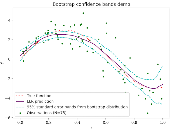
We present error bars for a function estimated by local linear regression by the bootstrap method. The data exhibit heteroskedacity: the magnitude of noise increases with \(x\). Standard techniques may use a single, constant estimate of noise variance. In that case, error bands will be tighter in regions with more data, but this will not reflect the changing noise variance.

One strength of bootstrapping is revealed here. A computer can easily recompute a local linear regression estimate for each of the boostrapped samples. These will automatically vary more in regions of high variance. By repeating the process many times (here \(B=200\)) we compute 95% confidence bands by taking the 2.5th and 97.5th percentile of the set of boostrapped estimates at each point in the interval.

Observe that the confidence bands become wider not only at the edges, where there are fewer data points, but also towards the right where the data are noisier. It is worth pointing out that bootstrapping cannot help us get rid of a model's basic bias. At the maximum near \(x=0.3\) local linear regression is an underestimate. This is a basic issue with kernel averaging methods and may be addressed with, e.g., local quadratic regression or spline regression, but will not be solved with a resampling technique.

Conclusion

Computing a statistic by bootstrapping is a powerful and widely applicable technique. Perhaps its biggest advantage lies in its ease of implementation for a wide variety of statistical situations. The same statistics that are already being computed only need to be recomputed for the bootstrap samples.

References