gaussian process regression

Intro

In this document and accompanying Python script we study Gaussian processes and attempt to understand how they may be used for a particular supervised learning task, that is, suggesting a function that gives rise to the data so we can make predictions at a new points.

This is not a thorough exposition on Gaussian processes. I find it usefulto implement standard statistical and machine learning techniques "naively", that is, without using libraries like scikit-learn, to develop my understanding. Please feel free to see the accompanying script

The assumptions underlying Gaussian process regression (GPR) are similar to those in standard regression techniques (linear, polynomial, etc.) Let us start with an example and lay out the assumptions we make as we go on.

Example

We have data $\textbf{y} = y_1, \dots, y_n$ occuring at times $\textbf{x} = x_1, \dots,x_n$. Imagine there is some continuous function $f(x)$ underlying the data generating process, but measurements are noisy, so we have $$y = f(x) + N(0, \sigma^{2}_n)$$

Where the latter term is just noise from measurement error.

We build in intuitions about continuity by supposing that data points covary in a way that decreases with distance--proximal points have a high covariance and as the distance between points increases the covariance goes to zero. The choice of covariance function reflects our a priori understanding of the process that generates the data. We do better if we take into account expectations about periodicity, long-range effects, etc., however here we will use a simple and popular choice, and take an exponent of the squared distance, aka, the radial basis function kernel: $$k(x_i, x_j) = \sigma^{2}_m exp\frac{-(x_i - x_j)^2}{2 d^2}$$ $\sigma^{2}_{m}$ is the maximum covariance which occurs when $x_i = x_j$ $d$ is a scale parameter that controls how quickly covaraince decays with separation along the $x$-axis.

Data

We will generate some sample data using a simple functional form $$f(x) = \left(\frac{1}{3} (x-5)\right)^{2}$$ and take 20 inputs on the interval $[0,10]$, Add some random noise to the functions, representing measurement error, to get the observed data: $$\textbf{y} = f(\textbf{x}) + N(0, 0.25)$$ Now we compute some matrices which will facilitate sampling GPs that fit the data. First is $K(X_t, X_t)$, the covariance between all observed inputs.

K(X_t,X_t) =
[[k(x1,x1), k(x1,x2), ...]
[k(x2,x1), k(x2,x2), ...]
...]

Next we have $K(X_t, X_*)$, and its transpose, representing the covariance between the new inputs for which we make predictions and the observed inputs, and $K(X_*, X_*)$ which is just the covariance matrix for new input points, computed exactly as before. The definition of Gaussian process says that the (predicted) function values and the observed data points are distributed as a multivariate normal distribution. This distribution has covariance matrix composed of the matrices we computed earlier:

[y, y*] ~ Normal(0, K)

where $K$ is the matrix

[[K(X_t,X_t) + \sigma^{2}_{noise}I, K(X_t, X_*)],
[K(X_*, X_t), K(X_*, X_*)]]

We add noise along the diagonal of the observations covariance matrix to represent measurement error. The Gaussian process gives a distribution over functions, but in practice we only look at a finite set of new inputs $X_*$.

Prediction

I will not show the derivation, but the distribution of points at the new inputs, conditioned on the obseved data is another gaussian process, that is, a multivariate gaussian distribution with mean $$\mu(x) = K(x, X_t) [K(X_t,X_t) + \sigma^{2}_{noise} I]^{-1} y_t$$ Let's rewrite this equation to clarify some of its meaning. The vector $[K(X_t, X_t) + \sigma^{2} I]^{-1} \textbf{y}$ can be taken to represent weighted observations from the data. We can decompose the leftmost multiplication into a sum. Supposing we want to calculate the mean at $x'$, $$\mu(x') = \sum_{i=1}^{n} k(x', x_i) \textbf(y)$$ So our prediction at point $x'$ is given by a linear combination (with coefficients from the kernel) of weighted contributions from the original data points. We predict a value of y based on the vector of observations $y_t$. This vector is multiplied by the inverse of the covariance matrix, which is also called the precision matrix. Using the precision matrix to estimate a missing value by taking a linear combination of observations given by the precision matrix is the same as the interpolation step in simple kriging.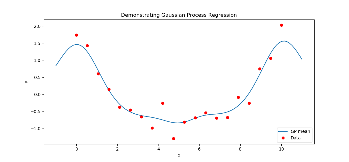

Gaussian process regression demonstration

Conclusion

With Gaussian process regression we can estimate the function at new inputs by treating the mean function $\mu$ as our best estimate of the underlying data generating process. However, the Gaussian process is really a distribution over functions, and we can get more information (e.g., confidence bands) if we use the fully specified Gaussian process rather than just the mean.
I will write more about this, and the other aspects of GPR which are neglected here later. We will discuss the choice of kernel, of hyperparameters, and the derivation of "useful" expressions like $\mu(x)$.

References

Ebden, M. "Gaussian Processes for Regression: A Quick Introduction." arXiv preprint (2015).
Schulz, E., Speekenbrink, M., Krause, A. "A tutorial on Gaussian process regression: Modelling, exploring, and exploiting functions." Journal of Mathematical Psychology (2018).